Review: Neural Rendering
Contents
- Introduction
- A Bit of History
- Forward Neural Rendering
- Inverse Neural Rendering
- Conclusion
- Aknowledgement
Introduction
Because rendering is such a massive topic, I’d like to start the conversation with some clarification.
As far as this article goes, rendering can be both a forward and an inverse process. Forward rendering computes images from some parameters of a scene, such as the camera positions, the shape and the color of the objects, the light sources etc. Forward rendering has been a major research topic in computer graphics. The opposite of this process is called inverse rendering: given some images, inverse rendering reconstructs the scene that was used to produce the input images. Inverse rendering is closely related to many problems in computer vision. For example, shape from X, motion capture etc.
Forward rendering and inverse rendering are intrinsically related because, the higher levels of a vision system should look like the representations used in graphics. We will look into both forward and inverse rendering in this article. In particular, how neural networks can improve the solutions to both these problems.
A Bit of History
However, before diving into deep learning, let us first pay a quick visit to the conventional approaches.
This is a toy example of ray tracing, a widely used forward rendering technique. Imagine we are inside a cave. The red bar is the light source, and the grid is the image plane. Ray tracing works by tracing a path from an imaginary eye through each pixel and calculating the color of the objects that are visible through the ray.
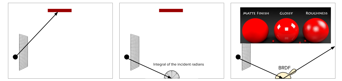 Figure 1: Ray Tracing.
In the left picture of Figure 1, the path reaches the light source, whose color is assigned to the pixel. But more often than not, the path will hit an object surface before reaching the light source (the middle, Figure 1). In which case the algorithm will assign the color of surface to the pixel. The color of the surface is computed as the integral of the incident radians at the intersection point. Most of the time these integrals have no analytic solutions and have to be computed via Monte Carlo Sampling: some samples are randomly drawn from the integral domain, and the average of their contributions are computed as the integral. To model different surface materials, reflectance distribution functions are used to guide the sampling process (the right, Figure 1). These functions decide how glossy or rough the surfaces are.
Most of the time, a ray needs multiple bounces before reaching the light source. Such a recursive ray tracing process can be very expensive. Different techniques have been used to speed up the process. To name a few: next event estimation, bidirectional path tracing, Metropolis Light Transportation … etc. I will skip all of them due to page limit. In general, Monte Carlo ray tracing has high estimator variance and low convergence rate. This means a complex scene will need hundreds of millions, if not billions, rays to render. For this reason, we ask the question whether machine learning can help us speedup Monte Carlo ray tracing.
As we will see later in this artile, the answer is YES. But before we dive into the answer, let’s quickly switch to inverse rendering for a second. I am going to use shape from stereo as a toy example (left, Figure 2). The algorithm takes a pair of photos as the input, and produces a reconstruction of the camera poses P0 and P1 and scene geometry. The first step is to find similar features between the photos. With enough matching, we can estimate the camera motion between these two photos, which is often parameterized by a rotation and translation. Then we can compute the 3D location of these features using triangulation. More photos can be used to improve the quality of the results.
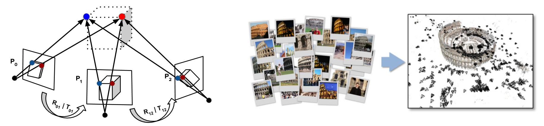 Figure 2. Left: Shape from stereo. Right: 3D reconstruction from one million images using bundle adjust, a technique invented by Sameer Agarwal et al.
Advanced technique can scale up to work with thousands or even hundreds of thousands of photos (right, Figure 2). These photos were taken under a wide range of lighting conditions and camera devices. This is truly amazing.
However, the output point cloud of such computer vision system is usually very sparse. In contrast, computer graphics applications usually demand razor sharp details. So in film and game industry, human still have to step in to polish the results, or handcraft from scratch.
Everytime when we hear the word “handcrafting”, it is a strong signal for machine learning to step in. In the rest of this article, We will first discuss how neural networks can be used as sub-modules and an end-to-end system to improve forward rendering. We will also discuss neural networks as differentiable renderers which opens the door for many interesting inverse rendering applications.
Forward Neural Rendering
Neural Networks as Sub-modules for MC Ray Tracing
First, let’s see how neural networks can help as a sub-module that speeds up Monte Carlo ray tracing. As mentioned earlier, Monte Carlo ray tracing needs many samples to converge. You can find an concrete example here1.
I’d like to make a fuzzy analogy here. You probably have heard of AlphaGO, which uses a value network and a policy network to speed up the MC tree search: the value network takes the board position as its input, and outputs a scalar value that predicts the winning probability. In other words, the value network reduces the depth of the search. The policy network similarly also takes the board position as its input, but it outputs a probability distribution over the best moves to take. In other words, the policy network reduces the breadth of the search.
The analogy I am going to make here is that there is also the value based approach and the policy based approach for speeding up Monte Carlo rendering.
For example, the value network can be used to denoise renderings with low sample per pixel. We can also use policy networks to make the rendering converge faster.
Neural Denoising for Monte Carlo Ray Tracing
Let’s first discuss the value network approach. Figure 3 demonstrates a recent technique for denoising MC renderings:
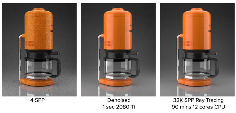 Figure 3. Adversarial Monte Carlo denoising with conditioned auxiliary feature modulation. B Xu et al. Siggraph Asia 2019.
On the left is the noisy input image that was rendered with only 4 samples per pixel. In the middle is the output of the denoiser. On the right is the ground truth rendered with 32k spp. The ground truth image takes 90 minutes to render with a 12 core intel i9 CPU. In contrast, the denoiser only takes a second to finish the rendering with a commodity GPU – a very good trade off between speed and quality.
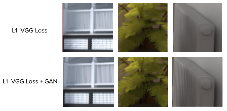
The denoiser network (Figure 4, left) is based on the auto-encoder architecture trained with L1 loss on VGG features maps, plus adversarial loss for retaining sharp details. And this2 is a comparison between training with and without the GAN loss. The one with adversarial loss is clearly better in recovering the details.
 Figure 4. Left: Network architecture for B Xu et al. Siggraph Asia 2019. Right: Elementwise biasing and scaling for injecting auxiliary features.
There are many literature about denoising natural images. However, denoising MC rendering is unique in a few ways:
Frist, one can separate the diffuse and specular components, so they go through different paths of the network, and the outputs are merged together. Studies found this gave better results in practice.
Second, there are inexpensive by-products, such by-product include albedo, normal, and depth maps, that can be used to improve the results. One can feed them into the network as auxiliary features. These features give the network further context where the denoising process should be conditioned on.
Finding an effective way to use auxiliary features is an open research question. We used a method that is called element-wise biasing and scaling (Figure 4, right): Element-wise biasing transforms the auxiliary features through a sequence of convolutional layers, and add the output to X. One can prove that it is equivalent to feature concatenation. Element-wise caling runs multiplication between the input X and the auxiliary features. The argument of having both biasing and scaling is that they capture different relationships between two inputs: intuitively, biasing functions as a “OR” operation that checks if a feature is in either one of the two inputs, where scaling functions as a “AND” operation that checks if a feature is in both of the two inputs. Together they allow auxiliary feature to be better utilized in the denoising process.
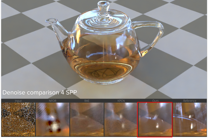
Here3 is a comparison between the neural denoising method and alternative methods at 4 SPP. As you can see, the neural denoiser method produces less artifacts and better details.
One important aspect of video denoising is temporal coherence. Remember Neural Networks is a complicated nonlinear function, which may map input values that are close to each other to somewhere really far away in the output space. The consequence is that if we denoise a video frame by frame, there might be unpleasant flickering between the frames.
To improve the temporal coherence, one can use a recurrent architectur4. At each time step, the network does not only output a denoised image, but also a hidden state \(h\) that encodes the necessary temporal information accumulated from the past. This hidden state, which is highlighted by the orange box, is fed into the network to denoise the next frame.
Neural Importance Sampling
So far we have been talking about denoiser as the value based approach. Now let’s take a look at the policy based approach.
Neural importance sampling is a technique invented at Disney research. the idea is that, for every location in the scene, we’d like to have a policy that guides the sampling process so the rendering converges faster.
In practice, the best sampling policy we can ask for an arbitary location is the incidence radiance map at that location. Because it tells you where the lights come from. The question is, how to generate such incidence radiance map for every location in the 3D scene?
Neural importance sampling (Figure 5, left) found an answer in the generative networks literature. Just like how image can be generated from vectors randomly sampled from a normal distribution, incidence radiance map can be generated from a vector of surface properties, including the coordinate of the intersection, the normal of the intersection, the direction of the incoming ray etc. The generative network is trained to map these surface properties to the incidence radiance map.
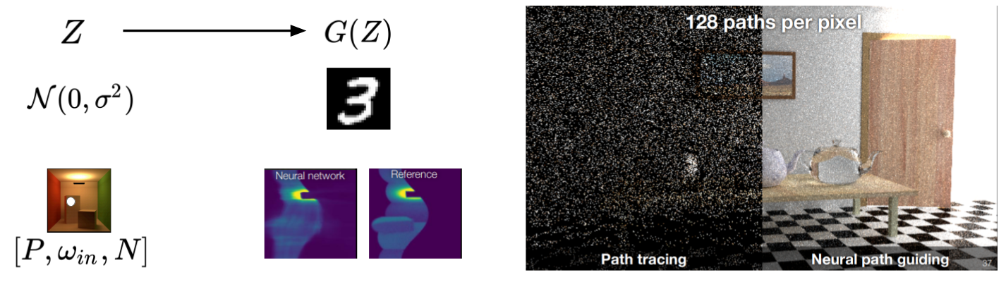 Figure 5. Neural importance sampling, Thomas Müller et al. ACM Transactions on Graphics 2019.
One unique challenge is the mapping between the surface properties and incidence radiance maps varies from scene to scene. So the learning of the policy network is carried online during the rendering. Meaning the network starts from generating random policies, and incrementally gets better at understanding the scene, and produces more efficient policy accordingly.
Figure 5, right is a side-by-side comparison between a regular ray tracing and the ray tracing with neural importance sampling. You can see at low samples per pixel, neural importance sampling is able to achieve much better result.
Neural Networks as an End-to-End Forward Rendering Pipeline
So far we have been talking about neural networks as sub-modules for Monte Carlo ray tracing. Next, we will use it as an end-to-end solution.
Recall ray tracing (Figure 6, left), which casts light rays from pixels to object surfaces. This is an “image centric” approach.
There is a different approach called rasterization (Figure 6, right), which cast rays from object surfaces to pixels. This is an “object centric” approach.
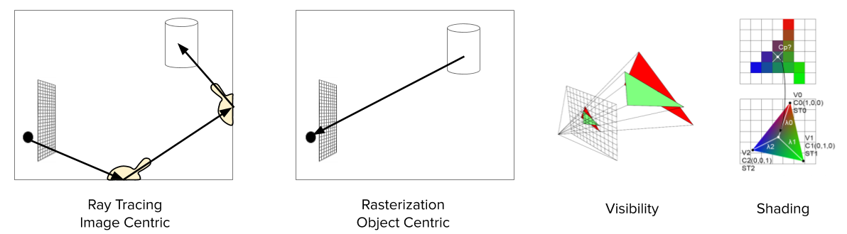 Figure 6. Left: Ray Tracing. Middle: Rasterization. Right: Compute visibility and shading.
There are two main steps in Rasterization: compute visibility and compute shading (Figure 6, right). To compute visibility, we impose the projected primitives on top of each other based on their distance to the camera, so the front-most objects can be visible. The shading process computes the color of each pixel. It does so by interpolating the color of the vertices.
Rasterization is in general faster than ray tracing because it only use primary ray. It is also easier for neural networks to learn because it does not use sampling or recursion.
All sounds great except that data format can also be a deal breaker here.
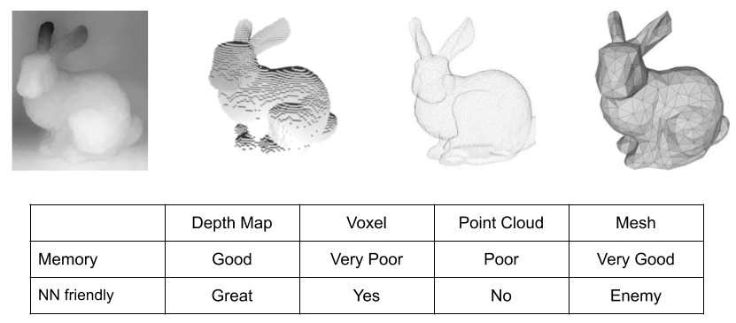 Figure 7. Popular 3D data formats.
Figure 7 shows the major 3D data formats for 3D models: depth map, voxels, point cloud and mesh. The truth is some of them are not friendly to neural networks.
Depth Map
Let’s start with the depth Map. Depth map is probably the most the easiest one to use. All you need to do is to change the number of input channels in the first layer, then it is good to go.
It is also memory efficient – the mainstream deep learning accelerators are designed to consume image data. So there is no problem here.
In the meantime, with depth map you get visibility for free. As all the pixels in the depth map come from the front-most surfaces. So the rendering only need to concern the shading.
There are many literatures5 about rendering depth map. I am not going into details here due to the page limit.
Voxels
Next, the voxels. Voxels are also friendly to NN as voxels are stored in a grid. However it is very memory intensive – it requires one order of magnitude more space than image data. As the result current neural networks can only process low resolution voxels. What is really interesting about voxel data is that it requires to compute both visibility and shading. So there is opportunity to build a true end-to-end solution for neural voxel renderer.
 Figure 8. RenderNet: A deep convolutional network for differentiable rendering from 3D shapes. T. Nguyen-Phuoc et al. NeurIPS 2018.
We tried this idea of end-to-end neural voxel rendering called the RenderNet (Figure 8). It started with transforming the voxels into a camera frame. I want to quickly mention that 3D rigid body transformation is something we do not want the network to learn. We will come back to this later but for now, just saying, 3D rigid body transformation is something really easy to do with coordinate transformation but very expensive to do with NN. We will come back to this later.
Once the input voxel is transformed into the camera frame, we use a sequence of 3D convolutions to encode it into a latent representation. We call this latent representation neural voxels (Figure 8, output of the orange block), where each voxel stores a deep feature that is used to compute visibility and shading.
The next step is to compute visibility (Figure 8, red block). One might be tempted to use the standard depth-buffer method. However it is not straight forward for neural voxels. First, the sequence of 3D convolution has diffused values inside the entire grid space, so it is hard to define what is the front-most surface for computing visibility. Second, each voxel stores a deep feature instead of a binary number. So the projection needs to integrate values across multiple channels to work out the visibility.
As the solution, RenderNet uses something called the projection unit. The projection unit first reshape the neural voxels from a 4D tensor to a 3D tensor by squeezing the depth dimension and the feature dimension. This is followed by an multilayer perceptron that learns to compute visibility from the 3D tensor. In essence, projection unit is an inception layer that does smart intergration across the depth and feature channels.
The last step computes shading with a sequence of 2D up convolutions (Figure 8, blue block). The entire network is trained with mean squared error loss.
Figure 9 shows some results. The left picture shows RenderNet learns to produce different shading effects. The first row shows the input voxels. The second row is the Phong shading results created by RenderNet. As you can see, RenderNet is able to compute both the visibility and the shading correctly. The rest rows of this picture shows that RenderNet can be trained to create different types of shading effects, including contour image, toon-shading, and ambient occlusion. In term of generalization performance, We can also use RenderNet trained on chair models to render new, un-seen objects, for example, the bunny (middle, Figure 9). RenderNet is also able to handle corrupted data (the 2nd row) and data with lower resolution (the 3rd row). The last row renders a scene with multiple objects. Last but not the least, RenderNet can render objects in different poses and scales (right, Figure 9).
 Figure 9. Results of RenderNet. Left: RenderNet can learn to produce different shading effects. Middle: RenderNet trained with chair models can generalize to work with corrupted data, low-resolution data and complex scenes with multiple objects. Right: RenderNet can render an objects from different views and is robust to scale.
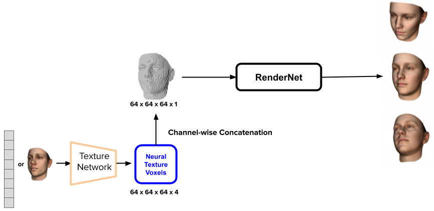
RenderNet can also render textured model6. To do so we use a texture network to create a neural texture voxels that can be channel-wised concatenated with the input binary shape voxel. The concatenated voxel is then used as the input of the network.
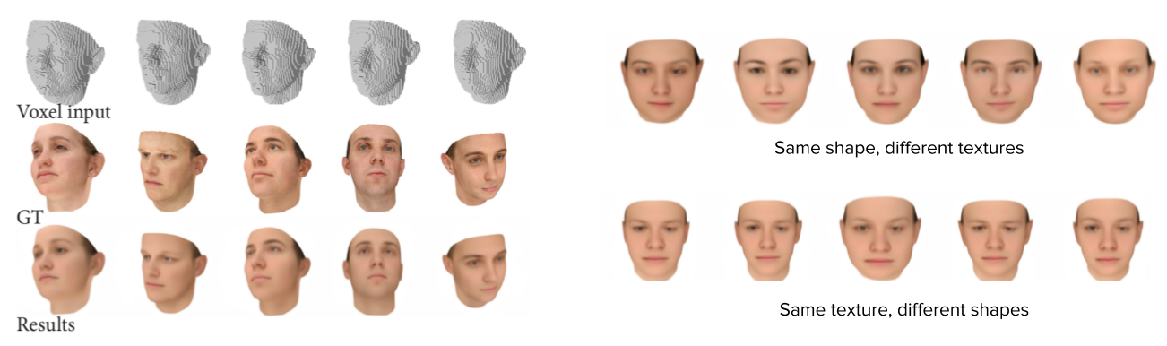 Figure 10. Results of rendering textured model using RenderNet. Left: comparison with ground truth rendering. Right: mix-and-match shape and texture inputs.
Figure 10 left are some rendering results with comparison to ground truth reference images. The ground truth images are obviously sharper than the rendered results. We think this is due to the fact that only MSE pixel loss was used to train RenderNet. However, the main facial features are well preserved by the RenderNet. Figure 10, right shows that we can also mix-and-match the shape input and the texture input. The first row shows the results rendered with the same shape input but different textures input. The second row shows the results rendered with different shape inputs but the same texture input
Point Cloud
Next, we have the point cloud. Point cloud is not so friendly to neural networks because it is not arranged in a grid. Especially, the number of samples and the order of samples can also vary, which is not ideal for neural networks. Similarly to voxel, we need to compute both the visibility and the shading.
First, let’s see how conventional rasterization is done for a point cloud: To compute visibility, each 3D point is projected into a square on the image plane. The side length of a square is inversely proportional to the depth of the 3D point. These squares are imposed onto each using the conventional Z-buffer algorithm. In the shading stage, once can simply use the colour of the 3D point to paint the squares. Due to the sparsity of the pointcloud and the naive shading process, the result image is often full of holes and colour blobs.
One interesting technique to improve the result is the Neural Point-Based Graphics method invented by researchers as Samsung AI lab7. The key idea is to replace the RGB color information with a learnt neural descriptor. A neural descriptor is an eight-dimensional vector associated with each 3D point. These information stored in the neural descriptors compensate the sparsity of the point cloud. You can see the first three PCA components8 of the neural descriptor in this image. The descriptors are randomly initialized for each 3D point. Since they encode information from a particular scene, they have to be optimized in both the training and the testing stage.
An autoencoder is used to render the neural descriptors. During training, the rendering networks is jointly optimized with the descriptors. During testing, the rendering networks is fixed, but the neural descriptors has to be optimized for each new scene.
Here8 are some results, which I think are truly amazing. The cool thing about the neural descriptor is that they are trained to be view invariant. Meaning you once optimized, the point cloud can be rendered in arbitrary views.
Mesh
Last, we have the mesh. The graphical representation makes it really difficult for neural network to deal with. But I do want to quickly point out a couple of works
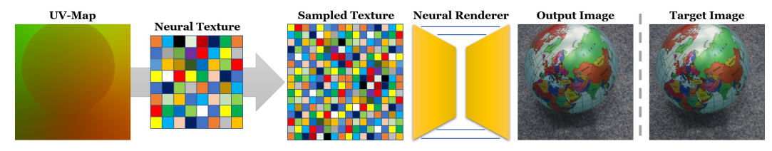
The first work is the Deffered Nerual Rendering9 technique invented by Thies et al. It is very similar to the neural point cloud method we just talked about, which learns a scene-specific “neural descriptor” that improves the conventional RBG based point cloud rasterization. Differently, they did this for mesh models. In particular, their method learns an object-specific “neural texture” that improves the conventional RGB based UV map for low resolution polygon models.
Another work is this very cool paper called “neural mesh renderer”10, which is able to do 3D mesh rendering, as well as 3D neural style. However, their neural network is mainly used to deform a mesh and change its vertex color. The rendering process is largely based on the conventional rasterization method hence is not particularly “neural”.
Inverse Neural Rendering
So far we have been talking about NN for forward rendering. It is time for us to switch to inverse rendering. Given an image, inverse rendering tries to reconstruct the scene that produced that image. We have mentioned shape from stereo with a toy example.
In general, inverse rendering is a very challenging task because every pixel depends on many parameters and there are a lot of ambiguities in the reconstruction. Here we will talk about a particular solution to this inverse problem called differentiable rendering.
Differentiable Rendering
This is how differentiable rendering works:
 Figure 11. Differentiable rendering for model reconstruction.
With a target photo, we can start from an approximate of the scene. This approximation does not need to be very good. All we need to do is being able to render the approximation and compare the result with the target. We can define a loss that quantifies the difference. If the render is differentiable, we can backpropagate the gradient of the loss to update the model. And we do this iteratively until the model converges.
The key is that the rendering function has to be differentiable. However, this can be difficult for conventional rendering engines. For example, Monte Carlo integration has discontinuity based on the distribution of the samples, which can make conventional ray tracing nondifferentiable.
Let’s see what parameters in a path tracer are differentiable, and what are not.
Recall path tracer relies on Monte Carlo sampling, which generates random samples within the intergral domain and computes the average of their contributions (Figure 12, left). Let’s use a toy example to illustrate this process: The square represents a zoomed-in pixel in the image plane. The dots are the random samples. Monte Carlo integration uses the mean of these samples, \(E\), as the estimation of the pixel value. At the sametime, we let \(E\) to be the output of a (rendering) function with input parameters \(P\), such as the geometry and the colour of the surface. Differentiable render requests the partial derivative of \(E\) with respect to \(P\) to be computable. The question is, is this true for Monte Carlo Rendering?
The answer is YES, sometimes.
Let \(P\) be the surface color (Figure 12, left). One way to check whether such partial derivative is computable is to see if changing \(P\) causes continuous changes to \(E\). In this case, the anser is YES: if all samples intersect with the same surface, then the same color change is applied to all the samples. If samples are from different surfaces, then the change of \(E\) is a linear combination of the changes from different surfaces, weighted by the number of samples intersects with each surface. In both cases, the derivative \(\frac{\partial E}{\partial P}\) is computable.
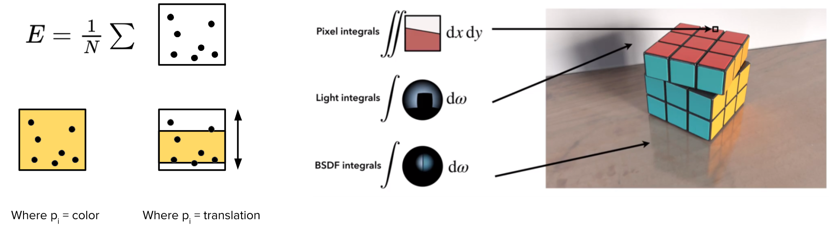 Figure 12. Analysis on the differentiability of Monte Carlo ray tracing. Left: Monte Carlo Intergration is differentiable to the change of surface colour, but not to the change of surface location. Right: Such non-differentiability exists for pixel intergal, light intergal and BRDF integral. Image source: Reparameterizing Discontinuous Integrands for Differentiable Rendering, G. Loubet et al.
Now, let \(P\) control the location of a surface (Figure 12, left). As a toy example, let a yellow surface “cut” across the integral domain (the pixel), and \(P\) to control the vertical translation of the surface. As we move the yellow surface vertically, it will miss or hit the samples, causing \(E\) to be discontinuous and non-differentiable with respect to \(P\).
Such discontinuities caused by changing the location, or in general the geometry, of the objects are everywhere in a physically based rendering. Not only in pixel integrals but also in light integrals and BRDF integrals. For example, moving an object can change the shadows and the reflections in the scene (Figure 12, right).
A lot of effort has been devoted to make physical based rendering differentiable. For example, one can add samples around the discontinuities (surface edges) to compute unbiased estimations of partial derivatives (Figure 13, left). However, this technique requires computing silhouette edges that creates discontinuities, which are expensive to do for complex scenes.
Another approach that does not involve computing silhouettes is to move the samples with the discontinuity (Figure 13, middle). Howevers, when a scene changes, it is rarely the case that all surfaces will move in the same way. So it is non-trivial to move the samples in such a way that they can follow the changes of the discontinuities in the scene. In which case the assumption of local coherence has to be made in order to have this method work.
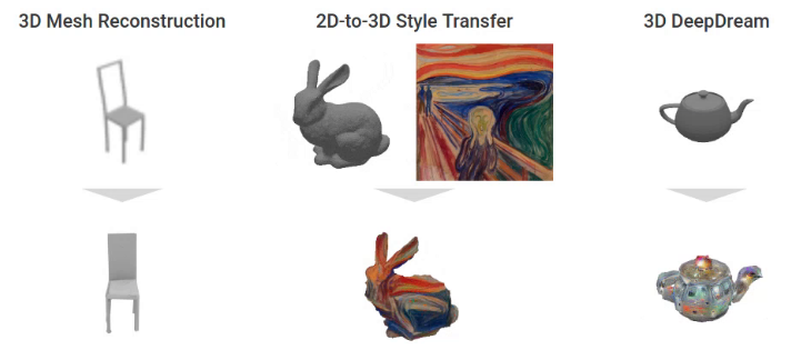
Finally, one can also modify the (step) integral function to be gradual (Figure 13, right). This idea was implemented as a differentiable mesh rasterization technique10 that supports single image based mesh reconstruction and 2D-3D style transfer.
In summary, differentiable rendering is non-trivial due to the sampling process used in the conventional rendering techniques. Next, we will discuss neural networks as an alternative solution.
 Figure 13. Approaches to make Monte Carlo ray tracing differentiable. Left: Differentiable Monte Carlo Ray Tracing through Edge Sampling, Tzu-Mao Li et al. Middle: Reparameterizing Discontinuous Integrands for Differentiable Rendering, G. Loubet et al. Right: Neural 3D Mesh Renderer, H. Kato et al.
Neural Differentiable Rendering
Now, let’s switch to the neural networks based approach and you can immediately see its advantages.
First, modern neural networks are made to run back-propagation. This makes them very attractive for implementing differentiable renderers, because we basically get the gradient for free.
Secondarily, neural networks can speed up the inverse rendering process. Notice the iterative optimization can be expensive to run and oftentimes is not suitable for real time applications. What neural networks can do is to approximate the optimization as a feedforward process. For example, an autoencoder can be used to learn latent representation from images. These representation can then be used for many downstream tasks such as scene relighting and novel view synthesis.
Scene Relighting
Let’s use scene relighting as a concrete example. The basic idea of scene relighting (Figure 14) is to sample the appearance of a static scene under different lights, then synthesize the scene under a unknown lighting condition using linear combinations of the samples.
 Figure 14. Acquiring the Reflectance Field of a Human Face, P. Debevec et al. Siggraph 2000.
Here, \(I\) is the target appearance, and \(M\) is the light transport matrix where each column is a vectorized form of a captured image. \(L\) is the coefficients for linear combinations. Obviously this approach relies heavily on data capture and \(M\) is often very big (2048 images were used in the original P. Debevec paper).
So it will be great if there is a way to reduce the number of captured images while still maintain the expressiveness of the light transportation matrix. This should be possible because light transport is highly coherent, resulting in highly similar appearance between nearby views. In other words, there is a lot of redundant information in the nearby samples.
However, there are two problems:
First, it is non-trivial to find a sparse set of views that can represent the scene in the optimal way. Random samples obviously does not work. Methods such as clustering failed to provide satisfactory results due to the fact that they are decoupled with the rendering process.
Second, with only a handful of samples, it can be really difficult to have high quality synthesized result using linear combination. For example, if individual lights cast hard shadows, their linear combination will create ghosting effects. In contrast, the ground truth image does not such such hard shadows.
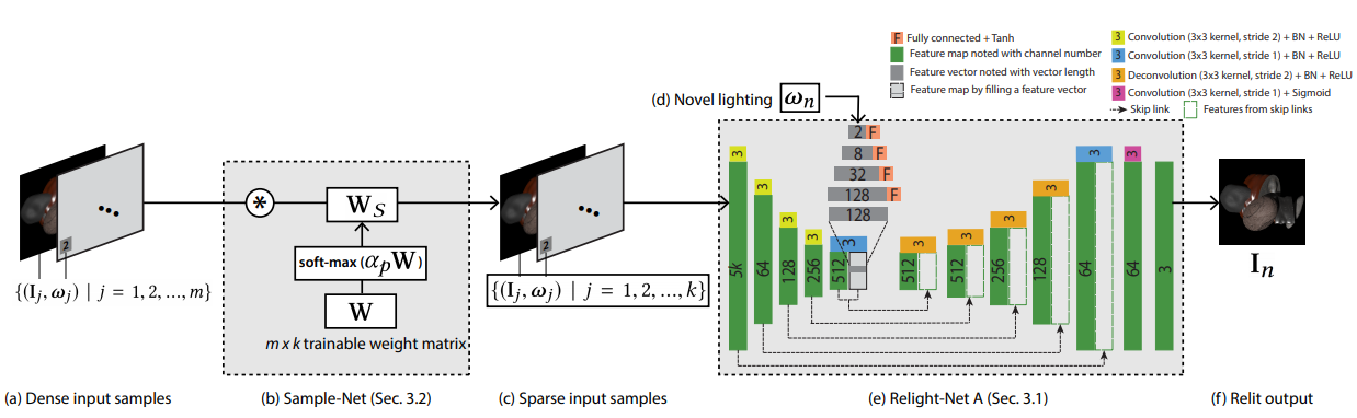
It turns out that both of these two problems can be addressed by machine learning. A recent work from researchers at UCSD and Adobe11 learns a sparse binary matrix to select a handful of images from hundreds or thousands of samples. A rendering network (autoencoder) then generates novel views from the selected images. The selection matrix and the rendering network are jointly trained to give the optimal results.
The result of this method is pretty awesome. However, it still needs to pre-generate a large number of samples for each scene for selecting the optimal views. The typical number of samples are between 256 to 1052, depending on the angular steps used for sampling. In the meantime, although one can synthesize the same view under different lighting, it is impossible to render the scene from a different view. In other words, it is designed to “compress” instead of “extrapolate”.
Representation Learning
A strong generative model is needed to draw reasonable scene images from a “prior” knowledge. To this end, a very interesting technique called “neural scene representation and rendering” was developed at DeepMind (Figure 15).
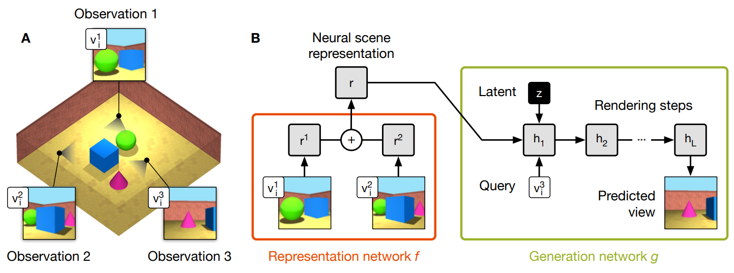 Figure 15. Neural Scene Representation and Rendering, S. Eslami et al. Science 2018.
The method can generate a strong representation of 3D scenes from very little or even no observations. For example, their network can predict novel views from only two input examples of the same scene (Figure 15, A). When no examples is given, the network is still able to use prior knowledge to generate meaningful images of random scenes.
The model contains a representation network and a generation network. The generation network (Figure 15, B) \(g\) uses a recurrent architecture to render a random vector \(z\) into a image. Using such a random vector as input allows unconditioned scene generation when there is no observation. The choice of a recurrent architecture, as the authors claim, is that a single feedforward pass was not able to obtain satisfactory results. In contrast, the recurrent network has the ability to correct itself over a number of time steps. Last but not the least, a query vector \(v\) is used to control the view of the generated scene.
In order to accomplish novel view synthesis of an existing scene, observations of the scene are used to condition the generation process. A representation network \(f\) is trained for exactly this purpose. It encodes an observation of a scene (an image) and its view parameters \(v\) into a latent representation \(r\). The generator \(g\) can only succeed if \(r\) contains accurate and complete information about the contents of the scene (e.g., the identities, positions, colours and counts of the objects, as well as the room’s colours). Multiple observations are aggregated by element-wise summing of individual representations. The the entire network is trained end to end to for novel new prediction.
The key assumption that makes this method work is that the representation network is forced to find an efficient way of describing the true layout of the scene as accurately as possible, since the generation network is constantly asked to predict images of unseen views during the training.
HoloGAN
In the context of machine learning, the assumptions used in the inductive reasoning process (build a model from the data) is often called “inductive bias”. One inductive bias I am very excited about is learning can be a lot easier if one can separate the appearance from the pose.
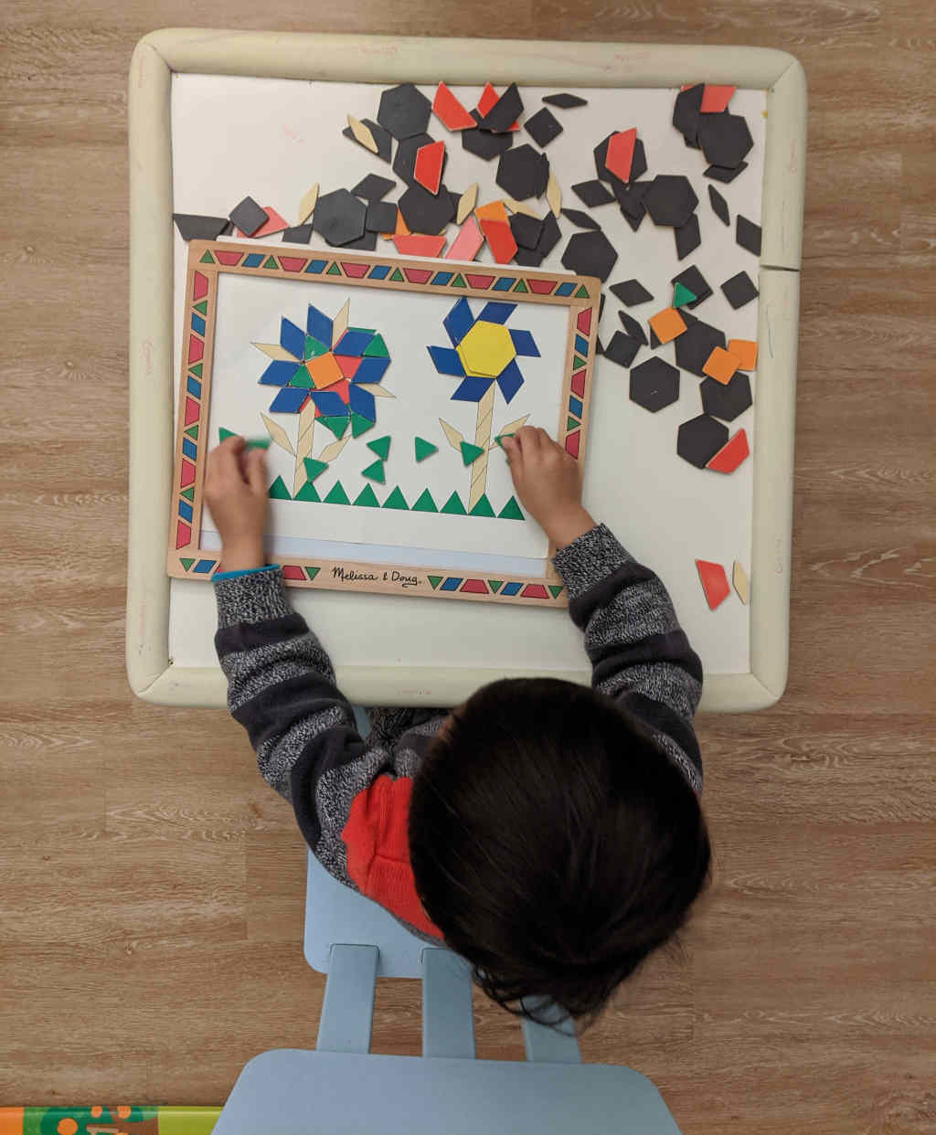
This is my four-year old son playing a shape puzzle. The goal is to build an object – in this case, the flowers, using some basic building blocks such as diamond, square etc. To achieve complete this task, he needs to apply rigid-body transformations to the building blocks before finding a good match on the board.
It is amazing to see this is something human can do with little or no effort. In contrast, most of the current neural networks are designed to struggle with it.
As a local operator, convolution is for sure not the right choice for (global) rigid body transformation. Fully connected layer may be able to compute it but at the cost of network capacity due to the need of memorizing all the different configurations.
So we wonder what if we just use conventional coordinate transformation to represent the pose, and separate the pose from learning the appearance of an object. Will that make the task easier?
We tried this idea in a recent work called HoloGAN. HoloGAN is a novel GAN network that learns 3D representations from natural images without 3D supervision. By no 3D supervision I mean no 3D shapes, no labels for camera view etc. The cool thing about this method is that learning is driven by the inductive bias instead of supervision.
 Figure 16. HoloGAN: Unsupervised learning of 3D representations from natural images. Thu Nguyen-Phuoc et al, ICCV 2019.
Conventional generative models12 use 2D kernels to generate images and make few assumptions about the 3D world. For example, conditional GANs using either feature concatenation or feature-wise transformation to control the pose of the objects in the generated images. Unless GT labels were used during the training, poses can only be learnt as latent variables, which can be hard to interpret. At the sametime, forcing 2D CNN to do 3D object rotation will create artefacts12 in the results.
In contrast, HoloGAN learns a better representations by separating the pose from the learning of the appearance. These13 are some faces randomly generated by HoloGAN. Once again, I’d like to emphasize that no 3D models or GT pose labels are used during the training. HoloGAN learns purely from 2D, unlabeled data.
The key is that HoloGAN uses 3D neural voxels (Figure 16) as its latent representation. Such a representation is both explicit in 3D and expressive in semantics, which improves the controllability and quality of the downstream tasks.
HoloGAN uses a 3D generator to generate neural voxels, and a RenderNet to render them into 2D images (Figure 17). The 3D generator is an extension of the styleGAN14 into 3D space. It takes two inputs: The first one is a learnt constant tensor. You can think of it as a “template” for a particular object category, such as human face, cars etc. It will be up-sampled to a neural voxel using a sequence 3D convolutions. The second input is a random vector as a “style” controller. It is mapped to the affine parameters for adaptive instance normalization throughout the entire pipeline.
The output of the 3D generator network (the neural voxels) is mapped to 2D images using RenderNet. For unsupervised learning, a discriminative network is used to classify the output of HoloGANs against randomly sampled real world images.
 Figure 17. HoloGAN architecture.
During training, it is crucially important to apply random rigidbody transformations to the neural voxels. This is how the inductive bias of 3D world is injected into the learning process: The network generates images from arbitrary poses not by memorizing all configurations but by generating a representation that is unbreakable under arbitary 3D rigid-body transformations. In fact, without this random perturbation, the network was not able to learn.
Let’s see some results: Here15 are some results on a car dataset. The method is pretty robust with transitions between views and complex backgrounds. Notice that the network can only generate poses that existed in the training dataset. For example, there is a relatively small range of elevation in the car dataset, so the network does not extrapolate beyond that range16.
However, the network is surely able to learn once there are more data comes in. For example, we trained the network with synthetic images rendered with ShapeNet models. The network is able to do 180 degree rotation in elevation[^hologan_chairs_ele].
We also tried some really challenging dataset. For example, the SUN bedroom dataset. This is extremely difficult to do because of the much bigger appearance variation across the dataset. As the consequence, the signal of pose is much weaker during the training process. We thought our method would completely break here. However, the result is very encouraging. For example, the main structure of the bedroom is very well preserved while rotating along the azimuth17. The elevation is more challenging probably due to the lack of examples in that direction18.
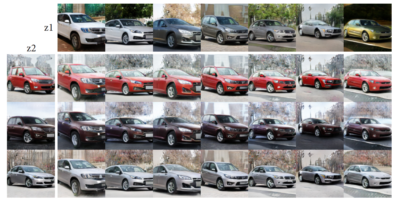
Another surprise is that HoloGAN seems to divide appearance further into shape and texture. To test, we can sample two random style control vectors, \(z1\) and \(z2\). If we feed \(z1\) to the 3D generator and \(z2\) to the RenderNet, we will see that \(z1\) controls the shape of the object, and \(z2\) controls the texture19: Every column in this image use the same \(z1\) but different \(z2\). So they have same shape but different texture. Every row in this image use the same \(z2\) but different \(z1\), so they have the same texture but different shape. To me this is really fascinating as it reminds me about the vertex shader and the fragment shader in graphics rendering pipeline, where the vertex shader changes the geometry and the fragment shaders changes the color.
Conclusion
Now it is probably the right time to draw some conclusion. We started the conversation by asking the question whether neural networks can be useful in forward and inverse rendering.
I believe the answer is yes.
As far as forward rendering’s concern, we’ve seen neural networks are used as both sub-modules and end-to-end solution. In the sub-modules cases, we can use NN as value networks or policy networks that reduce the depth and breadth of MC path tracing. In the end-to-end cases, NN have already shown promising results in rasterizing depth map, voxels and point clouds.
As to inverse rendering, we’ve seen neural networks as differentiable renders that learns strong representation for downstream tasks.
Before ending the discussion, I just want to say that neural rendering is still very much a research new field and there is a lot of space for you guys to make contributions. For example, there is still a big gap in terms of quality between physically based rendering and end-to-end neural rendering. As far as I know, there is no good solution for neural mesh rendering. Differentiable rendering opens a whole new door for representation learning, and it is really interesting to see how the community can push the learning forward with more effective inductive bias and network architecture.
Aknowledgement
I’d like to take the opportunity to thank the amazing colleague and collaborators who did increditable work in developing the techniques described in this article. In particular, Thu Nguyen-Phuoc who did most of the work for RenderNet and HoloGAN; and Bing Xu who developed the neural denoising technique for Monte Carlo Rendering. I also own much of the credits to Yongliang Yang, Stephen Balaban, Lucas Theis, Christian Richardt, Junfei Zhang, Rui Wang, Kun Xu and Rui Tang for their wonderful efforts.
-
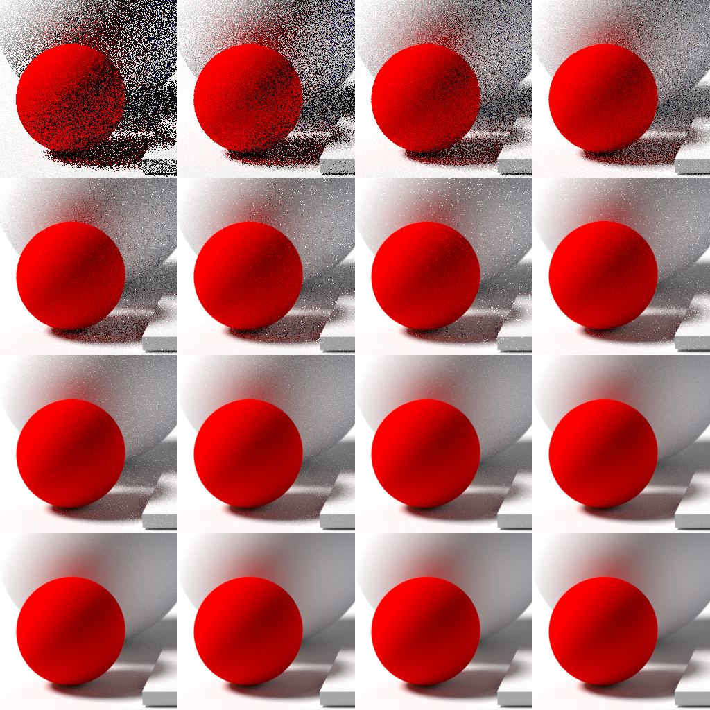 Noise decreases as the number of samples per pixel increases. Image Source: Wikipedia. The top left picture shows one sample per pixel, and doubles from left to right each square. Noise decreases as the number of samples per pixel increases. However, the computational cost also increases linearly with the number of samples, which motivates us to develop more efficient rendering techniques at a reduced sample rate. ↩
 -
Interactive Reconstruction of Monte Carlo Image Sequences using a Recurrent Denoising Autoencoder
 ↩
↩ -
Deep Shading: Convolutional Neural Networks for Screen-Space Shading O. Nalbach et al. EGSR 2017.
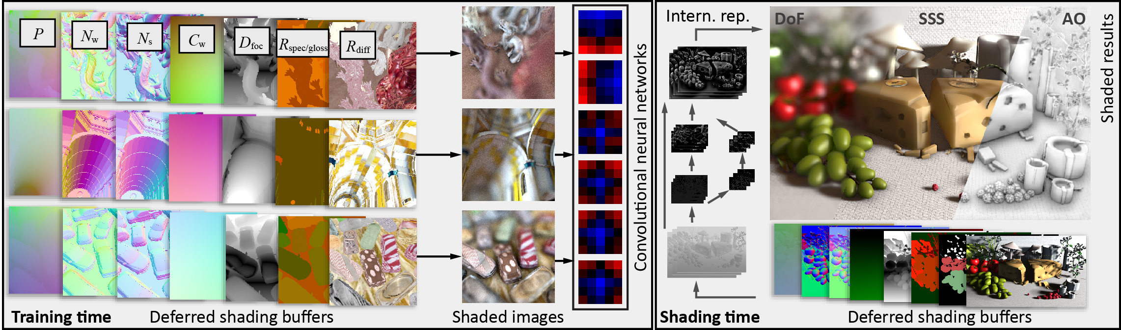 Image source: http://deep-shading-datasets.mpi-inf.mpg.de/ ↩
 -
Using RenderNet to render a textured model.
 ↩
↩ -
Neural Point-Based Graphics, Kara-Ali Aliev et al.
 ↩
↩ -
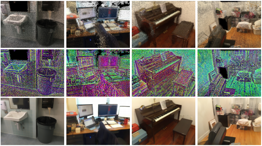 Image source: Neural Point-Based Graphics, Kara-Ali Aliev et al. The first row is point cloud rasterization using RGB colors. The second row is the visualization of the learnt neural descriptor using the first three PCA components. The bottom row is the rasterization using the learnt neural descriptors. ↩ ↩2
 -
Deferred Neural Rendering: Image Synthesis using Neural Textures
 ↩
↩ -
 Random faces generated by HoloGAN. ↩
 -
A Style-Based Generator Architecture for Generative Adversarial Networks. T. Karras et al. ↩
-
HoloGAN results: randomly sampled cars + azimuth rotation
 ↩
↩ -
HoloGAN results: randomly sampled cars + elevation rotation
 ↩
↩ -
HoloGAN results: randomly sampled bedrooms + azimuth rotation
 ↩
↩ -
HoloGAN results: randomly sampled bedrooms + elevation rotation
 ↩
↩ -
HoloGAN results: mixing shape and texture using different control vectors.
 ↩
↩
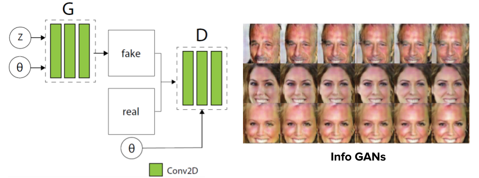 Conditional GAN and InfoGAN (X. Chen et al).